Avoid Errors in Excel: 6 Strategies of How to Prevent Mistakes

In our last article, we have seen the 5 biggest fails in Excel. But instead of laughing about these mistake, we should rather talk about how to find and avoid errors. In this article, we’re taking a look at 6 methods of how to prevent errors in your spreadsheet.

Method 1: Excel tells you – listen to it

In most cases, Excel tells you about possible mistakes. There are two ways: Indicating formula errors – like wrong cell ranges within formulas – with green corners or the more obvious by returning error messages.

1: Pay attention to the green corners 

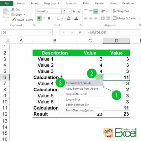
Have you noticed the small green corners of Excel cells? They indicate, that there might be something wrong with the formula. For example, it’s the only cell with a different range among the bordering cells. Microsoft says about these green corners:

A green triangle in the upper-left corner of a cell indicates an error in the formula in the cell. If you select the cell, the Trace Error button appears. Click the arrow next to the button for a list of options.

If you click on the trace error button, you’ll see what’s wrong with the cell. In the picture on the right hand side there seems to be an ‘inconsistent formula’.

2: Solve error messages 

Excel returns error messages like #N/A! or #VALUE! and so on. Take these errors seriously and solve them. If you are sure they won’t interfere with your results, you can hide them by using the IFERROR function. If you need help with such errors, please refer to our error helper: Select your error message and formula and you’ll get a detailed description of possible and probable cause and solution.

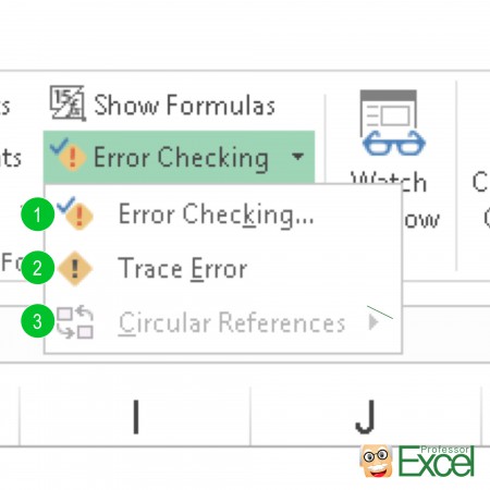
Within the formula auditing group on the Formulas ribbon, Excel provides tools for Error checking (the numbers are corresponding to the picture on the right hand side):

1.  Jump directly to the next error. You’ll get a short description of the error and options to solve it.
2. Trace Error visualizes the error path with arrows.
3. If you got circular references in your workbook, you can jump there if you click on ‘Circular References. For more information about circular references please have a look at this article.

Method 2: Avoid errors by checking sums

Checking sums is often troublesome as it requires additional work besides your actual calculations. But it is very useful. Let’s have an example: You got input data, then you conduct some calculations and finally got an output sheet with the final results:

• Use these results and compare the sums to the input data.
• Probably within your calculations, you filter or summarize the data. Use a simple filter on the input data to compare it to your results as well.
• The COUNTIFS helps checking if the number of data sets of the results matches to the number of input data and so on…

Furthermore try to judge:

• Do these results seem probable to you?
• Are there any outliers?
• Would you have expected such results? 
• What are the implications of such results?

Method 3: Display and check formulas

Besides the error checking tools as described before, Excel offers two other great tools within the ‘Formula Auditing’ group on the ‘Formulas’ ribbon:

1. You can display all the formulas instead of the resulting values. Click on ‘Show Formulas’ within the ‘Formula Auditing’ group (keyboard shortcut: Ctrl + `). When you select a cell, the input values will be highlighted.
2. Check the formulas – especially complex ones – with the ‘Evaluate Formula’ function. This tool let’s you follow up the calculations step by step. Select the cell and click on ‘Evaluate Formula’. Now press ‘Evaluate’ or ‘Step In’ as often as needed for checking each calculation step.

Method 4: Organize your workbook

It’s not directly a way to find and avoid errors in Excel, but in a clean and tidy workbook, it’s easy to get an overview and understand what’s happening. Furthermore – although it’s troublesome – try to write down your approach: Why did you choose this formula and why did you exclude certain values from your calculations. Some suggestions:

• Insert a list of open issues.
• Use a table of contents.
• Group worksheets by type, e.g. input vs. outputs. Please see the example below:

Method 5: Visualize your calculations and results

Even though your results might only be a table it can be helpful to visualize the data.

1: Insert a chart

Let’s say your results are monthly revenues: Display them in a simple bar or line chart. You can of course delete this chart afterwards but it gives you a good feeling about the results. For more information about how to insert a chart please refer to this article.

2: Add conditional formatting

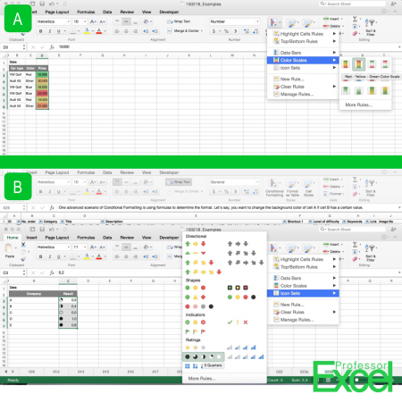
Another way would be using conditional formatting rules. Just select your data, calculations or results and click on ‘Conditional Formatting’ on the Home ribbon. A quick method is choosing color scales. The lowest values can be green and the highest in red. All the values in between will get shades of red and green. If you need more information about how to use conditional formatting please have a look at this post.

Method 6: Avoid errors by using named ranges

Using named ranges has two advantages and one disadvantage. Excel allows you to give names to cells and cell ranges. Just select the cell or range and type into the small text box on the top left corner of the screen (next to the formula bar). In your formulas, you can use the name instead of the reference. 

Let’s have an example: A tax rate is given in cell B2. You name this cell TaxRate. Now you want to multiply your net revenue (in cell B5) by the tax rate. Your formula now looks like this: =B5*TaxRate. This way, your formula is quickly readable and understandable. More importantly, you can avoid errors by not linking to wrong cells.