How to Hide Gridlines in Excel: 6 Expert Methods!

When you open a new Excel worksheet, it shows by default an empty table, just divided by thin grey lines. These grey gridlines are quite useful. They provide a quick impression of the rows and columns of your Excel worksheet. But once you want to finalize your layout, you worksheet or workbook often looks more professional without gridlines.

In this article we explore 5 methods of how to hide the gridlines in Excel. Furthermore, you learn how to hide them on all worksheets at once.

In a hurry? Go to the “View” ribbon and remove the tick mark from “Gridlines”. For more information, scroll down.

Contents

Method 1: Use white fill color for cells (strongly not recommended though)
Method 2: Change the color of the gridlines within the options menu (also not recommend)
Method 3: Just don’t let Excel display them (recommended)
Method 4: Hide all gridlines at once
Method 5: Hide all lines with a simple VBA macro
Method 5: One more method: Professor Excel Tools
- Also interesting:

Method 1: Use white fill color for cells (strongly not recommended though)

Unfortunately, this method can be found in practice quite often. Some Excel users “hide” the gridlines by using a white fill color. Although this way works – there are not any linesshown any longer – it’s strongly not recommended: Have you tried “restoring” the gridlines?

Method 2: Change the color of the gridlines within the options menu (also not recommend)

color, colour, gridlines, excel — You can change the color of gridlines

You can change the color of the gridlines. If you want to hide them, you can choose white color.

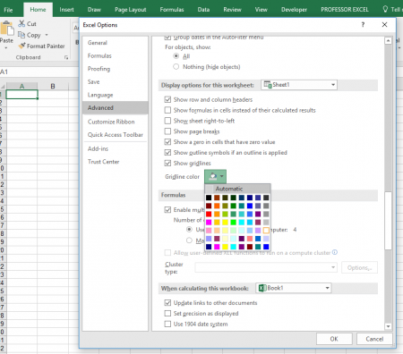
Click on “File” and then on “Options”.
Go to “Advanced”.
Scroll down until you see the “Gridline color” buttons. Click on “Gridline color”.
Select the color you’d like (or white) and confirm with OK.

Please note that you can only change the gridlines color of one worksheet at a time.

Method 3: Just don’t let Excel display them (recommended)

gridlines, gridline, hide, show, worksheets, worksheet, layout, excel

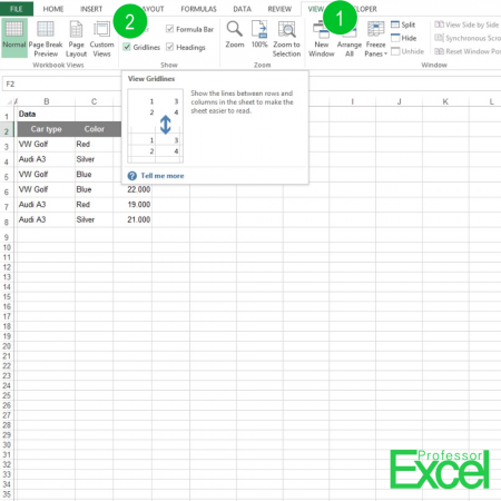
Usually, not displaying is the easiest and most professional way (the numbers are corresponding to the picture):

Go to the “View” ribbon and the “Show” group on the left side.
Untick “Gridlines”.

Method 4: Hide all gridlines at once

select, worksheets, once, excel — Select all worksheets at once

You want to remove the lines on all worksheets at the same time? It’s easy:

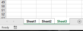
Select all the worksheet tabs. Therefore, click on one of the tabs, hold the Ctrl key and click on the other worksheets while still holding the Ctrl key. Alternatively, select the worksheet on the left (here: “Sheet1”) hold the Shift key on the keyboard and click on the furthest tab on the right (here: “Sheet3”).
Go to “View” and remove the tick mark from “Gridlines” (similar to method 3).

Do you want to boost your productivity in Excel?

Get the Professor Excel ribbon!

Learn more

Download Free Trial

Add more than 120 great features to Excel!

Method 5: Hide all lines with a simple VBA macro

In case the method 4 above is not working (maybe with older versions of Excel). Here is a simple VBA macro. Insert it into a new module (please see this article for more information) and press the start button.

Sub hideGridlinesOnAllWorksheets() 
    Dim ws As Worksheet 
    For Each ws In Worksheets 
        ActiveWindow.Sheets(ws.Name).Activate
        ActiveWindow.DisplayGridlines = False 
    Next ws 
End Sub

Method 5: One more method: Professor Excel Tools

layout, manager, gridlines, excel, tools, excel, add-in — For more comfort use the “Layout Manager”

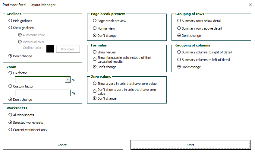
The Excel add-in Professor Excel Tools has a simple but powerful “Layout Manager”. It offers a variety of tools for easily applying layouts. If you open the layout manager you’ll also find the option of hiding all the gridlines in the whole workbook, on all selected worksheets or the currently active sheet only.