IFERROR: How to Handle Error Messages in Excel

When your formula produces an error in Excel – for example #N/A or #VALUE? – you got two options: Solve the error or use it in your calculation. Solving is usually a good idea but not always possible. So, let’s take a look at how to deal with errors in Excel formulas using the IFERROR formula.

What does the IFERROR formula do?

With the IFERROR formula you can define what to do in case of an error. Let’s say you got a “normal” calculation in cell A1: 

=B1/B2

What if B2 contains a 0 (zero) and B1 a numberic value? Your formula would return a #DIV/0! error message. Any formula using this output will now return #DIV/0! as well. That is troublesome, especially in large models, and above all doesn’t look good…

With the IFERROR formula you can define what to do in such case. For example, instead of showing the #DIV/0! error message, you can say “show 0” or do a completely different calculation (e.g. =C1/C2). The formula is especially useful in these cases:

• You want to avoid displaying error messages. Instead, you just want to leave blank cells or show a defined text.
• You can also use the IFERROR formula for a two step calculation. For instance, if you are searching for a distinct value via VLOOKUP in a list – if it’s not in this list (result is an error) you can define the next steps. For example looking it up in a second list.

How to apply the IFERROR formula?

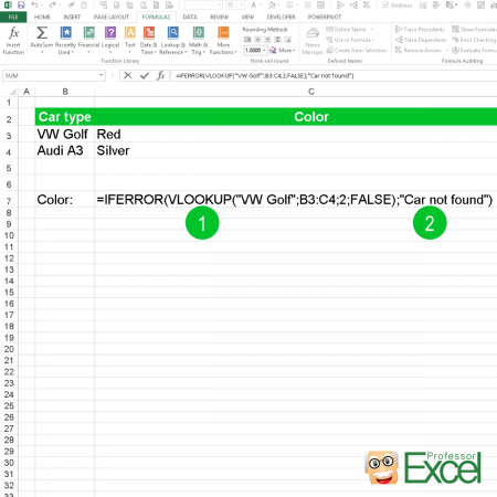
Applying the IFERROR formula is quite easy as it only has two parts (the numbers are corresponding to the image on the right hand side):

1. The first part contains the original formula or value. 
2. The second part defines what to do in case of an error. That could be a text, a number or another formula.

Usually you would start by just creating your original formula. If you then see that it produces an error you can wrap the IFERROR formula around it.

Let’s take a closer look at the example on the picture:

=IFERROR(VLOOKUP("VW Golf",B3:B4,2,FALSE),"Car not found")

In the middle, there is a VLOOKUP:

VLOOKUP("VW Golf",B3:B4,2,FALSE)

This VLOOKUP searches for the keyword “VW Golf” in the cell range B3 to B4. When found, it is supposed to return the color from column C (set by the number 2). Please refer to this article for more information about the VLOOKUP formula.

The VLOOKUP is wrapped within the IFERROR formula. That means, that if the keyword can’t be found, the IFERROR formula returns the value to be “Car not found” instead of an error message. Simplified:

=IFERROR(VLOOKUP(),"Car not found")

How to use the IFERROR formula on many different formulas at the same time?

Usually you can only add the IFERROR formula one by one around existing formulas. What if you’ve got to insert it on many existing formulas? 

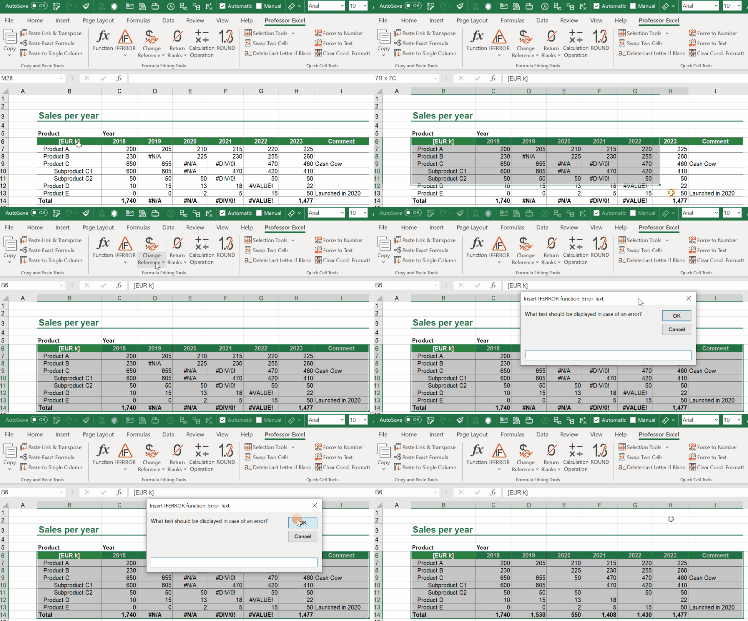
The Excel add-in ‘Professor Excel Tools’ provides an easy function for wrapping IFERROR around existing formulas: It literally just needs two clicks. Select all the formulas you want to edit and define what to do in case of an error:

1. Select all existing formulas and click on the button IFERROR within the ‘Quick Cell Functions’
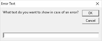
2. You’ll see the window on the right hand side. Now you can type the value or text you want to get in case of an error. Press OK to apply.

As the trial is free, no sign-up or installation needed (just activate it within Excel) you can simply download it by clicking the button below.