Merge Sheets: Easily Copy Excel Sheets Underneath on One Sheet!

Let’s assume you have many worksheets, all in the same structure. Or they are at least in a similar structure. Now, you want to combine them into one worksheet. For example copying them underneath each other so that you can conduct lookups or insert PivotTables. In this article, you learn four methods to merge sheets in Excel.

Method 1: Copy and paste worksheets manually

In many cases it’s probably the fastest way to just copy and paste each sheet separately. That depends of course on the number of worksheets you want to combine and their structure. Some comments:

• Try to use keyboard shortcuts as much as possible. For example for selecting the complete worksheet (Ctrl + A), copying the data (Ctrl + C), navigating to your combined worksheet (Ctrl + Page Up or Page Down) and pasting the copied cells (Ctrl + V).
• Also the shortcut of pressing Ctrl on the keyboard and clicking on the little arrow in the left bottom corner of your worksheet could help. That way you jump to the first or last worksheet in your Excel workbook.
• This method is especially useful if you just have to merge sheets once. If you need to do it repeatedly (for example you get new inputs every week or month) it’s probably better to check out methods 2 to 4 below.

Method 2: Use the INDIRECT formula to merge sheets

You can use Excel formulas to combine data from all worksheets. The main formula is INDIRECT.

This method has some disadvantages, though.

• The INDIRECT formula in general is slow because it’s volatile. That means, it calculates each time Excel calculates something.
• Using a combination of INDIRECT is usually unstable and error prone.
• It takes some work to set up the INDIRECT formula.

On the other hand, it has one major advantage: If you spend effort to set it up, this method is dynamic. That means when your input updates, the merged worksheet updates as well.

Approach

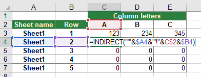
The INDIRECT formula can access any cell from a link (or better: an address) you provide. Please refer to this article to learn more about the INDIRECT formula. So you only have to provide the addresses for each cell in each worksheet you want to combine. Therefore, you should prepare a worksheet the following way (please refer to the screenshot on the right-hand side):

• Column A contains the sheet name.
• Column B contains the row number.
• Starting from Column C, you should add the column letters.

So let’s assume that you want to get the value from cell A1 of Sheet1. You would need then all the parts ‘Sheet1’, column ‘A’ and row ‘1’. Combining them in the INDIRECT formula would lead to the following formula. The formula in cell C4 is =INDIRECT(“‘”&$A4&”‘!”&C$2&$B4) .

Download

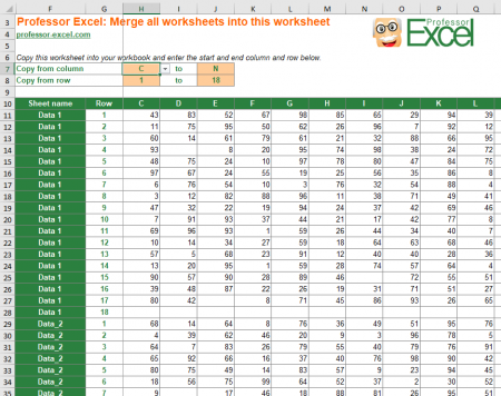
You want to save some time? We prepared a worksheet which can merge sheets automatically. What do you have to do? Download this workbook (~7 MB) and copy the only sheet into your own workbook. That’s it.

Please note the following comments.

• This method requires to enable macros (a list of all worksheets in your workbook is automatically created). When you want to save your workbook, you will be asked to switch to the XSLM file format.
• This model works for up to 50 sheets with 200 rows each (10,000 cells are prepared). If you need more, you have to extend it. The reason for this restriction is that the file is already quite large and requires some calculation performance.

Method 3: Merge sheets with a VBA Macro

You feel confident enough to use a simple VBA macro? Please insert the following code into a new VBA module. If you need assistance with VBA, please refer to this article.

Sub Merge_Sheets()
    'Insert a new worksheet
    Sheets.Add
    
    'Rename the new worksheet
    ActiveSheet.Name = "ProfEx_Merged_Sheet"
    
    'Loop through worksheets and copy the to your new worksheet
    For Each ws In Worksheets
        ws.Activate
        
        'Don't copy the merged sheet again
        If ws.Name <> "ProfEx_Merged_Sheet" Then
            ws.UsedRange.Select
            Selection.Copy
            Sheets("ProfEx_Merged_Sheet").Activate
            
            'Select the last filled cell
            ActiveSheet.Range("A1048576").Select
            Selection.End(xlUp).Select
            
            'For the first worksheet you don't need to go down one cell
            If ActiveCell.Address <> "$A$1" Then
                ActiveCell.Offset(1, 0).Select
            End If
            
            'Instead of just paste, you can also paste as link, as values etc.
            ActiveSheet.Paste
        
        End If
        
    Next
End Sub

Method 4: Combine sheets with “Professor Excel Tools”

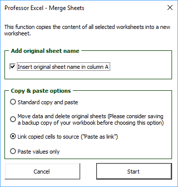
You like to use the most convenient way? Try the Excel add-in Professor Excel Tools.

• Just select all the worksheets you’d like to merge,
• click the button “Merge Sheets” and
• click on “Start”.

Alternatively, you can further refine your desired settings: Do you want to add the original sheet name in column A? No problem.

Also, define the copy & paste mode as shown in the screenshot on the right-hand side.

---

This function is included in our Excel Add-In ‘Professor Excel Tools’

Learn more

Download Free Trial

(No sign-up, download starts directly)

More than 35,000 users can’t be wrong.

---

(New) Method 5: Merge sheets using the Office clipboard

The first method above already dealt with copying and pasting sheets manually. There is one more trick here: Use the Excel clipboard to merge sheets. It’s actually quite simple, just follow these steps.

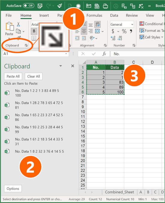
1. Open the clipboard: Click on the small arrow in the right bottom corner of the Clipboard section (on the Home ribbon).
2. Now you can see the clipboard.
3. Next, go through each worksheet. Copy all ranges which you later want to merge on one worksheet.

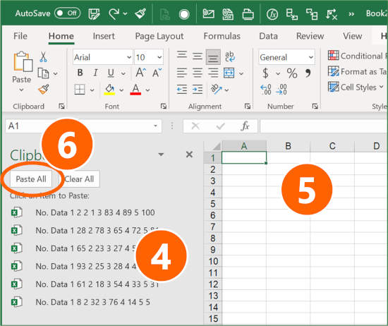
4. Now, you can see all your copied ranges in the clipboard.
5. Go to the sheet where you want to paste them underneath each other. Select the first cell.
6. Click on “Paste all”

That’s it. Especially with larger files, this method could save some time compared to method number 1 above. One small disadvantage: You can further adjust the pasting method, for example using paste special to paste values only.