
Usually you type =A1 for referring to the cell A1 in Excel. But instead, there is also another method: You could use the INDIRECT formula. The formula returns the reference given in a text. So instead of directly linking to =A1, you could say =INDIRECT(“A1”). In this article, we are taking a look at how to use the INDIRECT formula and why it is very useful. But there are also disadvantages.
Before we start: If you have already created an INDIRECT function and want to evaluate it, please refer to this article. It describes three methods to follow up INDIRECT formulas.
Steps for applying the INDIRECT formula in Excel
You want to get data from different sheets but always on the same cell?
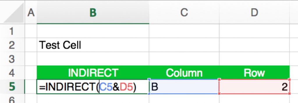
As said in the introduction, INDIRECT returns the value of a cell which you specify by a string. Please take a look at the picture on the right hand side. What will this formula return?
The function says
=INDIRECT(C5&D5)C5 has the letter B in it and D5 the number 2. If you combine them with the & sign, it’s B2. So if we step into this formula, it says =INDIRECT(B2). It refers to cell B2. As B2 contains the text “Test Cell”, the formula will return “Test Cell” in cell B5.
Do you want to boost your productivity in Excel?
Get the Professor Excel ribbon!

Add more than 120 great features to Excel!
Example: Use INDIRECT for referring to another sheet
Let’s take it a step further: Instead of just B2, you can also refer to other sheets, or even other workbooks. Let’s assume we type this formula into Sheet2 but we want to get the value from cell B2 on Sheet1. So, we have to add the worksheet name. This could look something like this:
=INDIRECT("Sheet1!B2")If you replace B2 with the cell references like in our picture, the formula will look like this:
=INDIRECT("Sheet1!"&C5&D5)Of course, you can now replace the static text “Sheet1!” by another cell reference, which contains the text “Sheet1”. Then you have to concatenate the cells including the ! in the middle. Please note that if your sheet names have spaces or special characters like “-” in them, you have to add ‘ before and after the sheet name:
=INDIRECT("'Sheet 1'!"&C5&D5)Example: Use named ranges in INDIRECT
Instead of creating cell references with the cell location, you can also use named ranges. Let’s assume you’ve named cell C6 “Tax_Rate” like in the following screenshot:
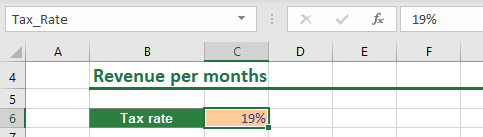
Now you can refer to this cell using =Tax_Rate.
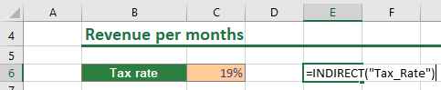
Using the INDIRECT function, it works the same way as with normal cell references: =INDIRECT(“Tax_Rate”). The name is not case sensitive, so it’ll also work when you type =INDIRECT(“Tax_rate”).
Why is the INDIRECT formula useful?
Within the reference of INDIRECT, you can combine the cell link as complicated as you like. If you have several similar sheets, for example filled out surveys. You can easily put together the indirect formula always linking to the same cells on each worksheet.
Furthermore you can use it within your formulas:
=VLOOKUP(A1,INDIRECT("Sheet1!A:B"),2,FALSE)There are countless ways of integrating INDIRECT into your formulas.
Disadvantages of the INDIRECT formula
Disadvantage 1: INDIRECT is Volatile
But there is are also disadvantages, especially in very large workbook: The INDIRECT formula is volatile. That means that Excel will calculate it again, each time when it calculates the whole workbook. Must other formulas will only be calculated depending on if their input values have changed. But INDIRECT will always be recalculated.
Disadvantage 2: Cell references not recognized by Excel
Another disadvantage is, that the reference is not recognized by a cell link. Let me give you an example: When you copy and paste a worksheet containing the INDIRECT formula, the break link function doesn’t work. Instead, you will see the #REF! error.
Also, formula auditing functions are hardly working: You can’t highlight the input cell with the “Trace Precedents” function. In the other direction it also doesn’t work: The the “Trace Dependents” function you can check, if your current cell is an input value for another cell. If your cell is an input for the INDIRECT formula, it won’t be detected.
Disadvantage 3: INDIRECT is very unstable
The formula is very unstable in terms of changing workbook structures. Most formulas adapt when you insert rows or columns. Or move cells.=A1 will adapt, when you move the cell A1. =INDIRECT(“A1”) on the other hand won’t.
Conclusion
The INDIRECT formula can be very helpful. It allows you to dynamically change cell references. But it comes with major disadvantages so that you should consider well, if it is worth using it.
How can I copy the value of cell A1 and paste said value into another cell, using the value of cell B1, to determine the cell location where the value is to be pasted?
Probably you’ll need a VBA macro for that. A good starting point would be recording a macro for copying and pasting a value (see this post: https://professor-excel.com/vba-macros-excel-record-edit-run/) and slightly change it so that the destination cell address is taken from cell B1.
I’ve got text in a cell (happens to be “b67”) but I want Excel to recognise that as a cell reference, so I can use it in formulae. Indirect will give me the Content of cell B67
Hi Colin, I’m not sure if I understand the question? Can you give me more information about this example?
Let us assume cell A67 contains the text “B67” and B67 cell contains 10. I want a formula to be written in C67 cell using A67 cell value to get 5 times of value stored in B67 so that the result is 50.
The formula in C67 should be =xyz(A67) * 5 which should be interpreted by Excel as = B67 * 5. Whereas xyz is an imaginary function. What is the formula to be used to achieve this?
I think I got it! Takes several formulas:
So, I have data on “Weekly Data” sheet and I want users to be able to enter a start and end date range, then select specified agents (from a drop-down list).
When the parameters have been entered, the formulas will look up this agent in the data sheet and add up (sum) the entries by that agent during that date range.
(If it helps the context, this is the number of calls taken by any given agent between dates.)
So…
User enters start and end dates for a lookup range (cells C3, C4).
Then I look up the rows for these dates – this finds exact match or next smaller (earlier) date:
=ROW(XLOOKUP(C3,’Weekly Data’!$A$4:$A$9999,’Weekly Data’!$A$4:$A$9999,,1))
Repeat for C4, but looking up exact or next higher (later) date:
=ROW(XLOOKUP(C4,’Weekly Data’!$A$4:$A$9999,’Weekly Data’!$A$4:$A$9999,,-1))
*My data is stored on a weekly basis using Monday dates
I then need to know the column reference for selected agents.
So in C7 the User selects staff names from a preset list, then this formula (located in F7) looks up the column for that individual:
=SUBSTITUTE(ADDRESS(1,MATCH(C7,’Weekly Data’!BC2:DZ2,1)+2,4),1,””)
*I actually allow users to select up to 10 agents in a table, so the looks ups repeat for each row with an agent name.
C7 is the first row in this “Agent Names” table.
If C7 is empty, the ‘total calls’ formula will return zero else will have the final ‘sum’ formula.
Almost there now!
In H7 I have the formula…
=TEXTJOIN(,,”‘Weekly Data’!”,F7,F3,”:”,F7,F4)
And finally in G7:
=SUM(INDIRECT(H7))
All these additional formulas/results will be hidden (I will either put them all in one column off to the side and hide it, or maybe have the font color white and lock the cells/sheet.
Hope that all makes sense! There’s probably an easier way, I am no expert, but it seems to work!
Can I refer to a cell using a title?
Meaning that I created a Vlookup function using big data. I have one row that has all the info from that big data. The first cell (A1) I created a listed names of all the accounts, so I can choose with out typing the names. Then I have created a second row named Total. Now I can compare each account with the total. Then, I added a chart to that table. So I can notice the results in the chart. However, now I am stuck, I wanted to name the title of the chart (Total Sales Compared with ” specific name account “.) Can I make the title change the name of an account based on A1? Meaning if A1 = Account blah. In the title will be (Total Sales Compared with “Account blah”.) if I change A1 to Account blah 2, the title change as well?
I wish my question is clear. Thank you.
Hi Malik,
If I understand your question correctly: yes, you can. You want to base a chart title on a cell content, right?
Just click on the title, then into the formula bar and type =A1. The chart title then shows the value of cell A1.
Best regards,
Henrik
Thank you so much for your help Henrik, I really appreciate it.
Hi Malik,
Thanks, I appreciate the “thank you”!
Have a great day,
Henrik
One more comment: I’ve updated the article with an example of how to use INDIRECT with named ranges… (although I think you won’t need it for your example…)
Let say the value of A1 is a word “sum”. Can I use indirect(A1) to as a function sum? Ex: indirect(A1)(A2:A4)
Is it possible to save a formula in a cell and refer to the formula as indirect reference to populate a value. I am having 5 formulas that will need to be replicated across all the data calculation grid according to some conditions. I would rather want to dynamically “build” and run the formula based on value saved in a template formula which can be referenced with an indirect call. Is it possible? Eg, instead of cell A1 having value 5, it may have a formula of =Row()*5. Is it possible to use this with indirect?
I’m trying to use the Indirect function to pull data from the same row referenced in a formula from a different worksheet.
“Sheet BMO” has a list of values in Columns A, B, C, and D
In “Sheet Summary”, A1 contains the formula =’BMO’!A3
I’m trying to create a formula in “Sheet Summary”, B1, that would use the formula in A1 and return the value from “Sheet BMO” D3, or offset 3 columns from A3.
I want to ensure that when I change the reference formula in “Sheet Summary” (=’BMO’!A3), the resulting value will also change to the applicable sheet and column/row.
Hope this is clear – appreciate any help I can get. I’ve tried Indirect and Offset in a variety of forms but can’t seem to get it to work.
I have this formula sumifs:($E1034:$KB1034;$E$893:$KB$893;”>=”&E411;$E$893:$KB$893;”=”&E411;$E$893:$KB$893;”<="&F411) so that it summs automatically?
Thank you
I need to create a template speadsheet on which people fill in any number of rows, from 0 to 50000. There will be a fixed number of columns.
I then want to be able to paste in a number of formulas below that will extract certain information, no matter what the number of rows.
The two variables I need are the first row of data and the last row of data.
Can I use indirect to create cell references within all the formula when I already know the column number, but the beginning and ending row numbers need to be two variables that are the same across all the formulas, while the columns differ? Would I need to put my formulas on a second page on the worksheet?
Am I making any sense?
Thank you so much!