
Working with percent values in Excel is very easy and convenient. In some cases, however, you want to work with per mille values. My impression: It was not really considered when Excel was developed. In this article, you will find three main methods, each with different options to insert per mil (or: parts per thousand).
Method 1 (fastest): Insert the per mille symbol ‰ into the cell next to your value
Our first method might not be as elegant, but it’s fast: You insert the per mille sign into a cell next to your value.
Please note: Your value, calculated by numerator divided by denominator, must be multiplied by 1,000.
1a) Use Professor Excel Tools
The fastest way to insert the per mille symbol: Use our Excel add-in Professor Excel Tools. As you can see, it only takes two quick clicks.
You can try it for free (no sign-up required). Download Professor Excel Tools here or learn more about the Excel add-in.
1b) Copy & Paste per mille sign from here
You don’t have Professor Excel Tools? No problem, here is how to insert the per mille symbol manually. The second fastest way is probably to copy & paste the ‰ sign from here:
‰1c) Insert the UNICHAR character with the Symbol function
As the last of the three options to insert the per mille sign, you can use the Insert Symbol function in Excel. The first time, it requires a few more steps but since then the ‰ symbol will be listed in the recently used symbols list.
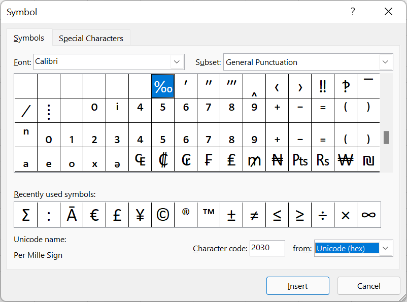
- Go to the Insert ribbon and click on “Symbol” on the right-hand side of the ribbon.
- Type “2030” into the “Character code: ” field and make sure that “Unicode (hex)” is selected in the from field.
- Click on Insert.
Method 2: Convert value to text and insert ‰ into same cell
The second method will show the per mille sign inside the same cell. Unfortunately, this converts the number to a text value and can therefore not be used in further calculations.
Copy and paste the following Excel formula and replace C4 and C5 by your numerator and denominator:
=C4/C5*1000&"‰"Do you want to further “fine-tune” the output? Then, use the slightly changed formula.
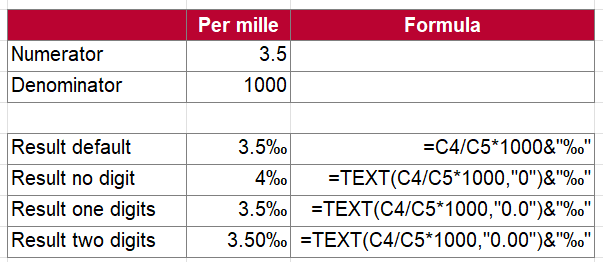
Use this formula for no digits:
=TEXT(C4/C5*1000,"0")&"‰"For one digit, use this formula:
=TEXT(C4/C5*1000,"0.0")&"‰"Use this formula for two digits:
=TEXT(C4/C5*1000,"0.00")&"‰"Method 3: Change the number formatting to per mille
The third approach is a combination of the first two methods above. The output is still a numeric value, but the ‰ sign is shown in the same cell through the formatting. To achieve this, two steps are necessary.
Step 1: Multiply by 1000
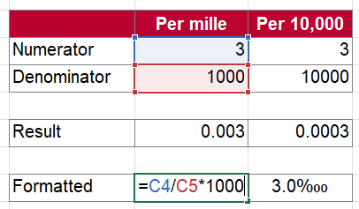
In order to display the values in per mille notation, you have to multiply them first by 1,000.
As you can see in the screenshot, it’s as simple as it sounds. So, the formula is
=C4/C5*1000Step 2: Add ‰ symbol in the number formatting
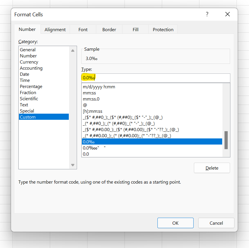
- Press Ctrl + 1 on the keyboard so that the Format Cells window opens.
- On the Number tab, go to “Custom” on the left pane. Copy and paste one of the following codes.
For no digits, type:
0‰If you want to display one digit, use this code (this one is shown in the example screenshot):
0.0‰For two digits, use this code:
0.00‰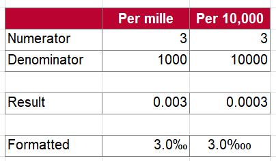
That’s it, confirm with OK and you are done. If you want to learn more about the custom number formats, please refer to the big guide.
Download

Please feel free to download all the examples above in one workbook. Click here to start the download.
Thanks the easiest way to get a ‰ symbol is type Alt + 0137, but as in Methods 1 and 2 this just gives you a text value that can’t be used for direct calculations [which is what I was hoping to find a solution for, in the same way that excel recognizes percentages] without additional unnecessarily complex manipulation (converting text back to a number).
Method 3, custom format is the best way to go if you want to both display in a single cell and use the the ‘per mille’ value in a calculation – simply divide the per mille figure by 1,000 within whatever formula you are writing.
[I didn’t really understand the point of your method of dividing by 1,000 to then multiply by 1,000 to get back to the starting figure, even if correctly formatted, to use it practically you would as stated above have to divide it 1,000 again to use in a formula]