Random Values in Excel: Everything You Should Know (+XLSX-Download)

Sometimes, you want to create random values in Excel. For example, when you want to simulate some kind of statistical distribution, make up random key codes or want to pre-fill some database. In this article, we’ll take a look at the two Excel formulas RAND and RANDBETWEEN with a lot of examples.

How to create random values in general

There is a simple formula to generate random numbers: RAND. If you type =RAND()  into a cell, you’ll get a number between 0 and 1.

Two comments:

1. The RAND formula has no argument. So don’t type anything between the brackets.
2. You’ll get many decimals. We’ll explore later on how to use that.

That’s the easy case – let’s take it a step further.

Create random values with decimals and between a minimum and maximum value

What do you do, if you want to have random number between 20 and 50 for example?

Use the RAND formula and do some maths: The interval is 30 (=50-20). We have to multiply =RAND() by 30. That means, the random number will be between 0 and 30. Now we only have to add 20. The result is then always between 20 and 50. If you want to create whole numbers, please add the ROUND formula.
In more mathematical terms: If you want to get a random number between a and b, you have to type

=RAND()*(b-a)+a 

Create random values without decimals (whole numbers) with a minimum and maximum value

If you want to get whole number you got two options: Either you use the method from our example before and wrap it into the ROUND formula with 0 decimals. Or you use the more elegant soluation: Use the RANDBETWEEN formula.

RANDBETWEEN works similar to RAND but has two arguments: the bottom (in our case 20) and the top value (in our example 50). The complete formula looks like this: =RANDBETWEEN(20,50) .

As said before: Please note that RANDBETWEEN only returns integer values. So if you some more decimals you should go with the first option.

---

Do you want to boost your productivity in Excel?

Get the Professor Excel ribbon!

Learn more

Download Free Trial

Add more than 120 great features to Excel!

---

Create even numbers with a minimum and maximum value

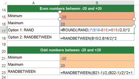
Let’s take a look at a special example. This example should provide an idea of how to solve more complicated cases. The example: You want to get an even number between -20 and +20.

Let’s set up the formula step by step using the RAND formula:

1. First you want to get a decimal number between the range 0 and 40 (that equals the distance between -20 and +20):
   =RAND()*40 
2. Next you move the range from “0 to 40” to “-20 to 20” by subtracting 20:
   =RAND()*40-20 
3. Now you already got a random number with decimals between -20 and +20. As the next step, you have to make it an even number. Therefore, you divide it by 2 and round it to 0 decimals. That way, you got a whole number between -10 and +10. Now you only multiply it by 2 . That’s it.
   =ROUND((RAND()*40-20)/2,0)*2 

There is also a slightly shorter way using RANDBETWEEN:

=RANDBETWEEN(-20/2,20/2)*2

One more note: If you want to get odd number, just add 1 in the end (and change the minimum and maximum values accordingly). So if you want to get an odd value between -20 and +20:

=RANDBETWEEN((B21-1)/2,(B22-1)/2)*2+1

Create normal distributed values

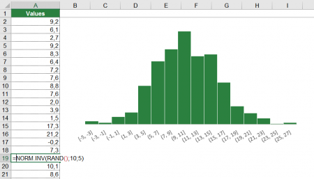
The RAND and RANDBETWEEN produce even distributed values. That means, each value between your minimum and maximum will come up with the same probability. Sometimes you don’t want that. Instead you want to get values with a distribution, let’s say the most popular normal distribution.

In such case you can combine the RAND formula with the NORM.INV formula. That way, you can create random values with a underlying normal distribution.

You need to specify:

• The probability (with the RAND() formula).
• The mean. This determines where the maximum is located.
• The standard deviation determines the width of the data.

If you put these input values together (let’s say with the mean of 10 and the standard deviation of 5), the formula looks like this:

=NORM.INV(RAND(),10,5)

Create random small and capital letters

You can also create random letters. Therefore you have to use a so-called ASCII code: Every character has a number (not only in Excel). Here is a list of ASCII codes. You only have to wrap CHAR formula around the RANDBETWEEN formula (with the correct minimum and maximum values). That way, Excel translates your random number into the corresponding character.

The formula for capital letters (they occupy numbers 65 to 90 among the ASCII codes):

=CHAR(RANDBETWEEN(65,90))

The formula for small letters:

=CHAR(RANDBETWEEN(97,122))

Final notes and download

Some more comments on both formulas (RAND and RANDBETWEEN):

• Both formulas are volatile. That means that every time when you recalculate your workbook, the random value will change. 
• Please note: RAND and RANDBETWEEN create even distributed numbers by default.
• Please feel free to download all the examples above from this direct download link.

Has this article helped you? Why don’t you subscribe to our free Excel newsletter?