Hide Zero Values in Excel: 3 Simple Methods

There are many reasons why you might want to hide zero values in Excel. For example when working with cell links, Excel shows a 0 even if the source cell is blank. Or because it might look more professional. Whatever reason you have, there are different methods for hiding zero values. Depending on the scope (for example one worksheet or just selected cells), different methods are most suitable. In this article we explore 3 methods of hiding zero values in Excel and compare them.

3 ways of hiding zeros in Excel

Let’s first take a look at 3 ways of hiding zeros in Excel. Then we compare them. Later on we take it one step further by learning how to blind out zero values in the complete workbook.

Method 1: Hide zero values with conditional formatting rules

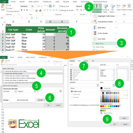
Probably the best known way: Using conditional formatting rules. Please follow these steps (the numbers are corresponding to the picture on the right hand side):

1. Select the cells or cell range in which you want to hide zeros.
2. Click on the ‘Conditional Formatting’ button in the middle of the ‘Home’ ribbon.
3. Click on ‘New Rule…’.
4. Now you’ll see a new window. Select the second list item ‘Format only cells that contain’.
5. Select the following values below: ‘Cell Value’, ‘equal to’ and ‘0’. This makes sure that all cells having a zero value will be formatted.
6. Click on the ‘Format…’ button in order to set the format.
7. Navigate to the ‘Font’ tab.
8. Click the small arrow next to ‘Color’ and choose a white font color.
9. Confirm with OK.

Please note that instead of really hiding zero values, conditional formatting can only apply white font color. In some cases, these values are still visible, for example when copying a table as an image to PowerPoint. Also, conditional formatting rules are always a little inconvenient to handle and maintain.

Method 2: Blind out zeros with a custom number format

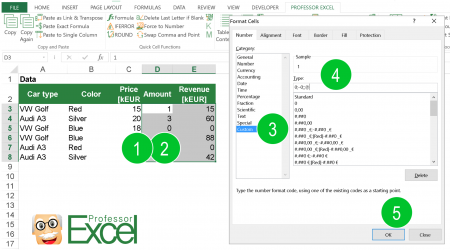
Another option for hiding zero values in Excel is using a custom number format. Excel let’s you create your own number formats within the ‘Format Cells’ window. Follow these steps:

1. Select the cells you want to format.
2. Press Ctrl  + 1  on the keyboard (or alternatively right click on one of the selected cells and click on “Format cells…”).
3. Click on ‘Custom’ on the left hand side.
4. Paste the code 0;–0;;@ into the ‘Type’ text box.
5. Confirm with OK.

Afterwards, you can apply further formatting. For example defining how many digits you want to display by using the corresponding buttons withing the ‘Number’ section on the ‘Home’ ribbon.

For more information about the custom number formats in Excel please refer to this article provided by Microsoft.

Method 3: Hide zero values within the worksheet settings

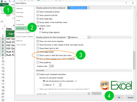
The third way is probably the most elegant way: Within the ‘Options’, you can untick ‘Show a zero in cells that have zero value’. But there are two disadvantages:

• It only works for all zero values on the selected worksheet. You can’t use this method for single cells or cell ranges.
  
• It only works for one sheet at a time.

Admittedly, this function is a little bit hidden within the Excel menu structure:

1. Click on ‘File’. On the left hand side click on ‘Options’.
2. Click on ‘Advanced’.
3. Scroll down until you reach the section ‘Display options for this worksheet:’ Select the desired worksheet. Next, remove the tick from ‘Show a zero in cells that have zero value’.

Comparison of the three methods

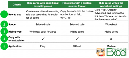
The question is: Which method to use in what case? The table on the right hand side might help with your decision:

1. Each method works differently – for detailed step by step guides please see the descriptions above.
2. The scope is important when deciding which method to use: If you want to format all zero values on the current worksheet, probably the third method (worksheet settings) is best for you.
3. Please be careful when using the first method (conditional formatting): Zeros are actually still shown – but only colored in white color. Sometimes when you copy tables to other programs, they might still be visible.
4. The first two methods you can copy and paste with the format painter.
5. These methods have different levels of difficulty: Because conditional formatting is probably the best known option, we classify it as easy. The second and third options are more hidden and therefore classified as difficult and medium.

Taking it one step further

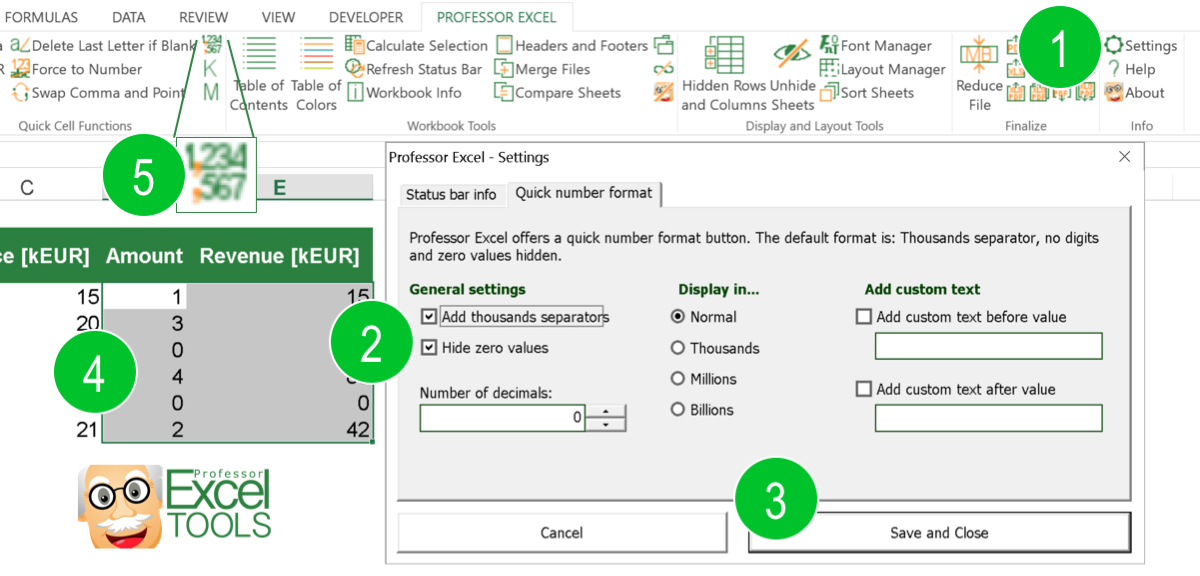
Because all these methods have major disadvantages, we included the option for hiding zero values into our Excel add-in ‘Professor Excel Tools’. There are two ways:

• Define your favorite number format or 
• use the layout manager.

Define your favorite number format once and apply it with just one click

Formatting numbers in Excel is very time consuming. Furthermore, some formatting options are not (easily) available. We believe, that you should spent more time on contents than on formatting. That made us come up with the option to define your favorite number format:

1. Click on settings within the ‘Professor Excel Tools’ ribbon.
2. Define your favorite number format, e.g. hide zero values. You can of course also set all the other preferred options like number of decimals our adding thousands separators.
3. Save by clicking on ‘Save and close’. You have to do these first 3 steps only once!
4. Select the cells you want to format.
5. Click on the button ‘Number’ to apply your preferred number format.

Define the layout for the complete workbook

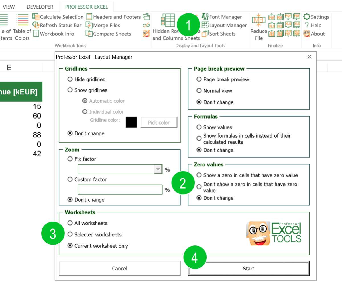
Many layout options Excel you can only apply sheet by sheet. Or they are very hidden. Therefore we added the function of setting the layout for complete workbooks. You only want to format some of your worksheets? No problem, select the sheets you’d like to format and start the layout manager.

1. Click on ‘Layout Manager’ in the center of the ‘Professor Excel’ ribbon.
2. Define your format. For hiding zero values choose ‘Don’t show a zero in cells that have zero value’.
3. Set the scope, e.g. all worksheets, selected sheets or just the current worksheet.
4. Apply it by clicking on ‘Start’.

All these functions are included in the Excel add-in ‘Professor Excel Tools’. Try it for free with the buttons below (no sign-up, no installation).

---

This function is included in our Excel Add-In ‘Professor Excel Tools’

Learn more

Download Free Trial

(No sign-up, download starts directly)

More than 35,000 users can’t be wrong.

---