The “Conditional Formatting” button is hidden in the middle of the Home ribbon in Excel. Nonetheless, Conditional Formatting offers many options for visualizing your data. As the name already says, Excel can format your table depending on one or more conditions.

In this Excel tip, we will take a look at two options of applying a format to your cells depending on a condition: Color scales and icon sets.
Conditional formatting with color scales
Color scales change the background color depending on the cell values. The default versions are the traffic light colors green, yellow and red. But there are also other options, e.g. blue-white-red (probably symbolizing cold to hot).

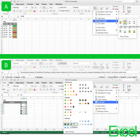
Figure (A) in the picture on the right hand side shows how to apply the color scale:
- Select a range of cells with values.
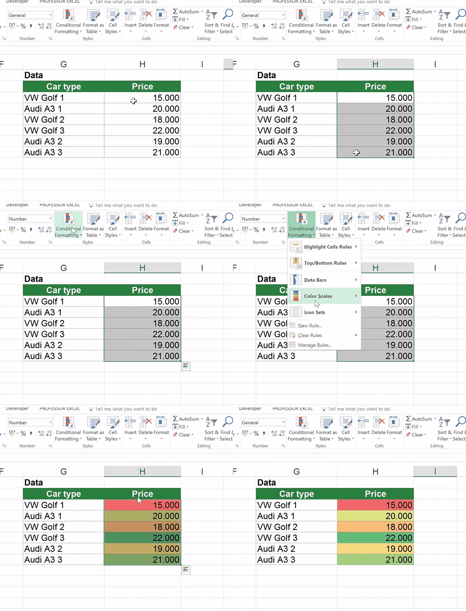
- Click on Conditional Formatting and then choose a scale under “Color Scales”.
Let’s say, we select the “Red-Yellow-Green Color Scale”. The cell containing the lowest value in your range will now get a dark green color. The cell with the highest value is dark red. All values in-between will have shades of green or red.
The animation above shows the opposite example: The lowest value get’s the red color and the highest value get’s green.
These color scales could be extremely useful for identifying and eliminating outliers.
Icon sets like traffic lights or harvey balls

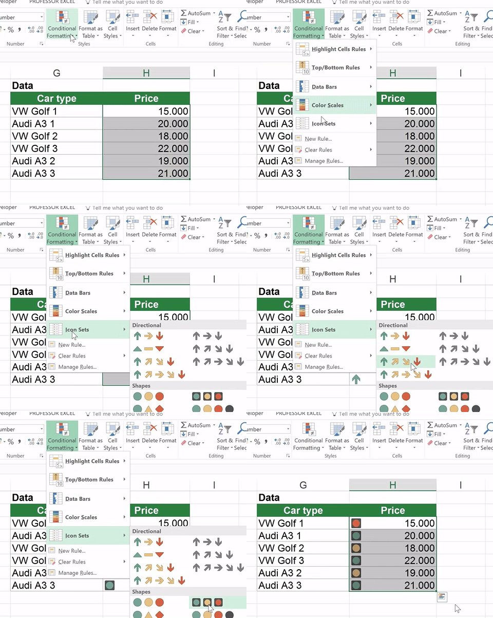
Instead of just background colors, you can add small symbols to the cells depending on their values: Such ‘icon sets’ can be traffic lights (red, yellow, green), arrows or Harvey balls (those quarter/ half/ three quarter filled circles). Please compare to figure (B) in the picture above.
In our example, we want to show achievements by using Harvey balls. Basically, it’s the same process:
- Select the data you want to visualize.
- Click on Conditional Formatting on the Home ribbon.
- Select Harvey Balls under Icon Sets.
Excel will now automatically calculate in which quarter each value belongs and add the balls to each cell.
Remove conditional formatting rules but keep the colors

In some cases, you want to remove the conditional formatting rules but keep the format. For example, you’ve selected the background color depending on the values (see above). Now you want to keep the color, but either delete the values or even change the values.
There is one very comfortable way: Use “Professor Excel Tools“:
- Select the cells having conditional formatting rules.
- Click on “Remove Cond. Formatting” within the Quick Cell Functions on the Professor Excel ribbon.
You can try the Excel add-in for free – no sign-up or installation needed. Just click the button below.

This function is included in our Excel Add-In ‘Professor Excel Tools’
(No sign-up, download starts directly)
More than 35,000 users can’t be wrong.
Final thoughts
- Conditional Formatting can use a lot of performance, especially when using with formulas. In case your computer suddenly gets noticeably slower, you might want to reduce the conditional formatting to a minimum.
- Use Conditional Formatting only when it really improves your table. Don’t just use it for adding colors to your worksheet.
Further reading
You want to know more about conditional formatting? Please take a look at our articles:
- If you want to use a formula for defining the format of a cell, please refer to this article. The example in this article: How to highlight all Sundays on a calendar sheet.
- You want to hide all zero values? There are several methods – one of them is via conditional formatting.

