Cell References Messed Up? How to Avoid Wrong Cell Links When Sorting in Excel

This problem is very annoying and not very reasonable: When you sort your Excel table, for example using filters, cell references messed up. Instead of linking to a cell in the same row, they suddenly refer to a cell in a different row. The dangerous part: Often, you want immediately notice it – and something like this might happen… Here is the reason and how to fix broken cell references after sorting data.

Summary

In a hurry? Here is the summary:

• Remove links to own worksheet before sorting an Excel table.
• Find & replace might be the fastest solution here.

Problem: Cell References Broken When Sorting Excel Tables

Admittedly, this is a curious problem. After you sort a table, the cell references within this table are broken.

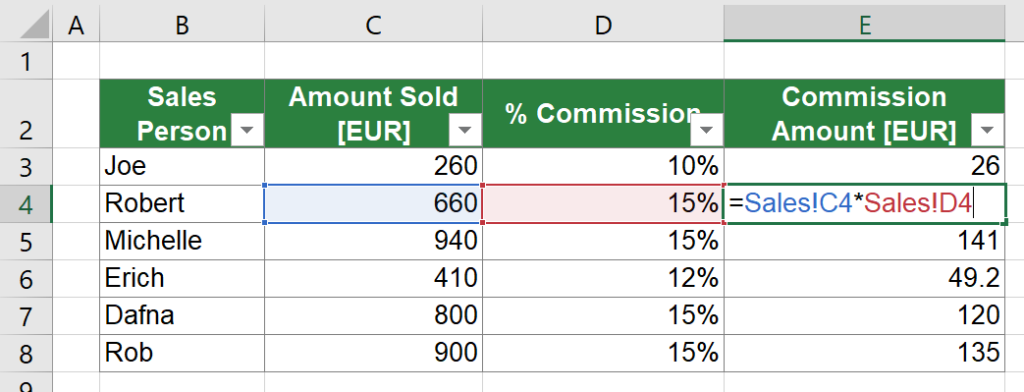
For example, your original table looks like this:

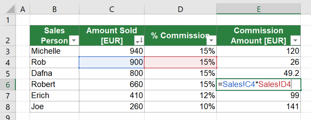
After you have sorted the table by the amount sold in column C, the function for Robert looks like this:

The solution, if cell references are messed up: Remove the worksheet name

The solution for this problem is quite simple: Remove the worksheet name from the cell reference. That way your links will adapt when sorting your table. So, instead of

=Sales!C4*Sales!D4

you just write

=C4*D4

Sounds simple, right? It has the further advantage that your formula is shorter and easier to follow up.

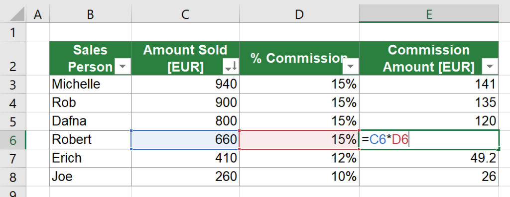
For our example from above, the solution would look like this.

Methods for removing worksheet references from cell links

Method 1: Removing the own sheet name in the reference manually

As usual, deleting the own worksheet name manually might be a fast solution. When you work with tables, you probably just have to do it once and copy & paste your function to all cell in the respective column.

Method 2: Use Find & Replace

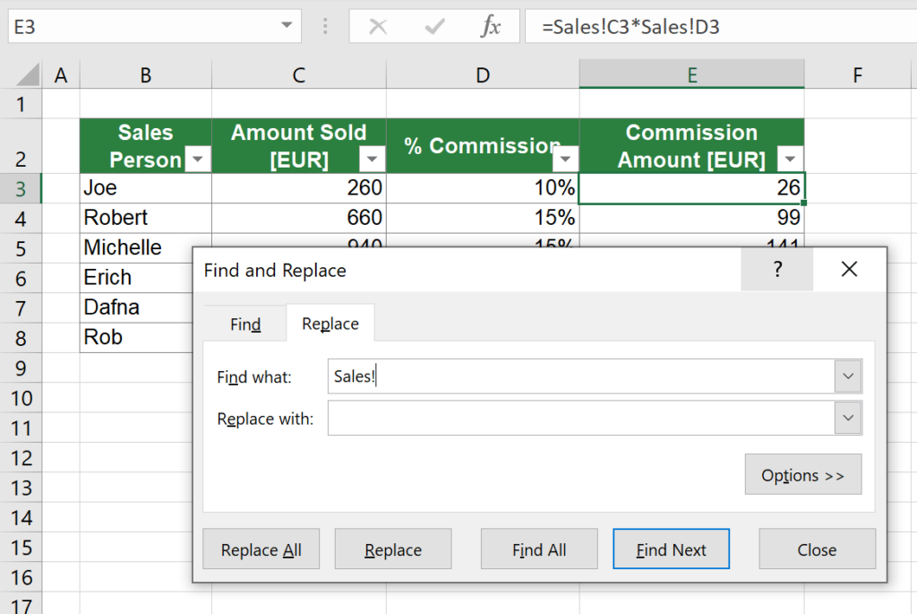
The find & replace function is quite powerful. Open it by pressing Ctrl + H on the keyboard. In the “Find what:” field you search for the worksheet name (in this case “Sales!”) and the “Replace with:” field you leave blank. Make sure to include the exclamation mark.

If something looks broken or you receive error messages after replacing the sheet names, you can undo it by pressing Ctrl + Z on the keyboard.

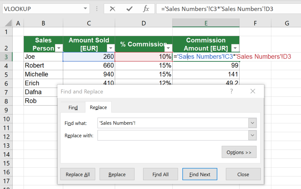
If your worksheet name includes a space (or any other special character – refer to this article for more information), also replace the ‘ characters. Excel automatically inserts the apostrophes when the sheet name has any of these special characters – and also removes them, when you rename your sheet (for example without spaces).

Method 3: Use Professor Excel Tools

The Excel add-in Professor Excel Tools has a built-in function to clean Excel functions and formulas.

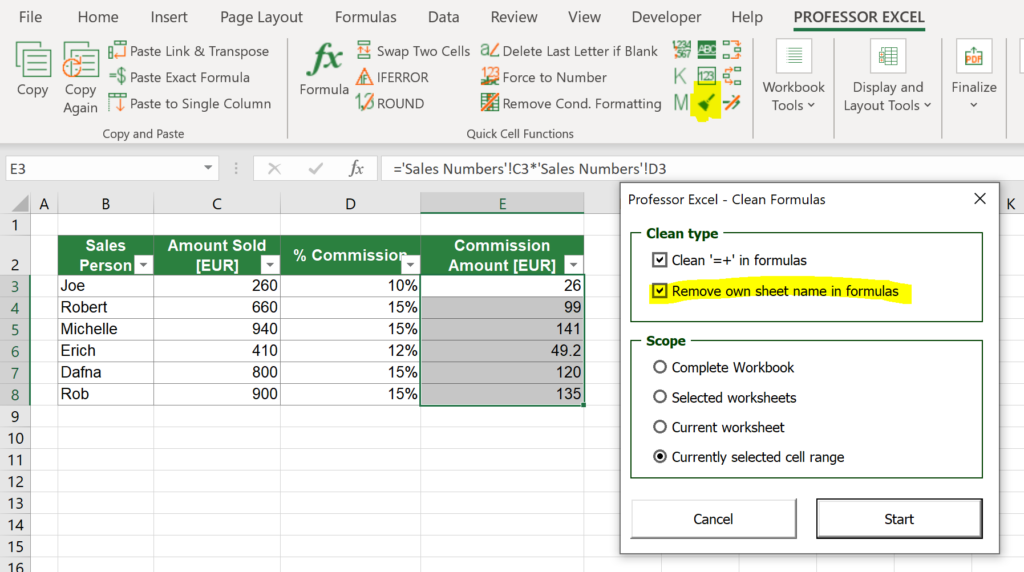
1. Select the formulas you want to clean.
2. Click on the brush symbol of Professor Excel Tools to open the “Clean Formulas” window.
3. Click on start.

Image by 412designs from Pixabay