How to Count Number of Unique Records in Excel: 5 Methods!

A common task in Excel is to find out the number of different entries in a list. For example, you have a list of names and want to know, how many different people are listed as some people might be multiple times on the list. This article introduces 5 different methods of counting the number of unique records in a list, regarding two major differences.

1. You simply want to know the number of unique records. You don’t need to consider any condition.
2. Or you want to know the number of different entries under one or more conditions.

Example for this article to count the number of unique records

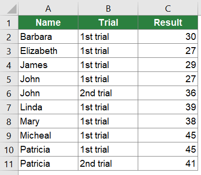
The screenshot on the right-hand side shows the example table. It is a list of ten persons contains three columns. The values are the results from a game a group of friends were playing. Column A has the name of the person, column B the number of trial and column C the result per person and trial. You want to answer two questions:

1. How many people were playing?
2. How many people had a result larger than 40 in the first trial?

Method 1. Using Excel function “Remove Duplicates”

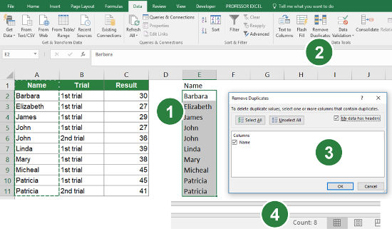
If you only want to count the number of unique records once and don’t have to automatically update the result, you could use the function called “Remove Duplicates”. It’s a built-in function in Excel and you can find it within the “Data”-ribbon.

1. Select the list or column you want to know the number of unique values of and copy it to a new sheet or empty space on the same sheet.
   Recommendation: Instead of simply pasting the cells, paste them as values by pressing Ctrl + Alt + V on the keyboard. Select “Values” and press enter. That way, formulas will be removed so that the values don’t change through possible underlying formulas within the pasting process.
2. Select the pasted values and click on “Remove Duplicates” on the “Data” ribbon.
3. A new window opens. If your data has headers, set the relating tick at “My data has headers”. Confirm with OK.
4. Select the list which now doesn’t have any duplicates any longer. In the bottom left corner of the window Excel shows the number of entries selected like this “Count: x”.

Alternatively, you could use the COUNT and COUNTIFS formulas.

Please note:

• Blank cells are ignored in the number in the bottom left corner of the screen.
• This method is not suitable for the second question of our example.

Method 2. Using advanced filters

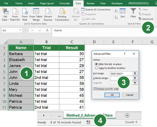
The next method—using advanced filters—works very similar to the previous method removing duplicates. Advanced filters in Excel provide a function to filter to unique records only. This advanced filter hides duplicates as you are probably familiar from normal filters. The screenshot on the right-hand side shows the steps.

1. Start by selecting the list or column containing the values you want to count the unique items from.
2. Click on “Advanced” within the “Sort & Filter”-group on the “Data”-ribbon.
3. In the new window check “Filter the list, in-place”, make sure the correct “List range” is selected and set the tick at “Unique reconds only”. Confirm with OK.
4. The status bar now shows already the number of records left. In this example it says “8 of 10 records found”.

Method 3. PivotTables

PivotTables are very powerful in Excel. Coming with the versatility, they are often complex to set up. In this part we take a rough look at the necessary steps to answer the questions using PivotTables. Because PivotTables could fill books themselves, we concentrate on the crucial steps rather than going too much into detail of all their basics.

PivotTables have the advantage that with an update of the data, they can be refreshed. Our previous methods 1 and 2 can’t be easily refreshed—at least not without going through all the steps again. On the other hand, PivotTables aren’t as dynamic as using Excel formulas.

Steps for creating the PivotTable and count the number of unique records

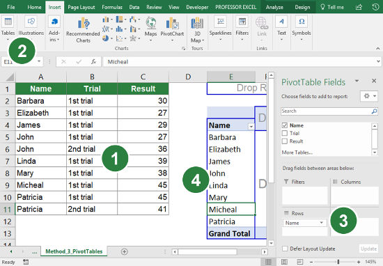
The necessary steps are shown in the image on the right-hand side.

1. Select your list or data.
2. Insert a PivotTable by clicking on “PivotTable” on the left-hand side of the “Insert”-ribbon. Follow the steps on the screen until the PivotTable is created.
3. Pull the column name you want to count into the “Row” field.
4. Select all names and look at the number shown in the status bar similar to the third step of the method 1 before.

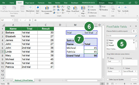
Answering the second question is a little bit trickier. The question is “How many people had a result higher than 40 in the first trial?”. You can use the same PivotTable you’ve just created for answering the first question and add some modifications.

5. Pull the column names “Trial” down into the Filter field and “Result” into the Values field.
6. Now use an overall filter to the data. Set the filter of “Trial” in cell N2 to “1st Trial”.You could use the same approach as in number 6 before for the result time. But the overall filter doesn’t
7. have advanced options like filtering all values larger than a given number. To achieve this, you need to use the Filter on the “Values” column. Click on the small arrow in the headline of the columns (here in cell M5). Define a Value Filter larger than 40. The result should look similar to the image above.

Method 4. Formulas SUMPRODUCT and COUNTIFS

The previous methods 1, 2 and 3 aren’t entirely dynamic. That means, with an update of the data, the results don’t automatically change without further steps. Even the PivotTable in our method 3 requires a refresh. Out methods 4 and 5 don’t have such constraints. They automatically update their results because they are based on Excel formulas.

Structure of the SUMPRODUCT / COUNTIFS functions

This method is based on the two Excel formulas SUMPRODUCT and COUNTIFS. For more information about these two formulas please refer to SUMPRODUCT and COUNTIFS.

The formula is comparatively short and works for up to one criteria. So, the second question of our example―as it requires two criteria―can’t be solved with this formula combination. In such case, please proceed with the following method 5.

The base formula combination is shown in the image above.

The COUNTIFS formula returns an array of numeric values. It has one value for each record of your data saying how many times it occurs. If one value only appears once, it will have the number 1. If it one the other hand appears twice, it will have two times 2. The &”” signs prevent blank cells (will be regarded as zeroes) to be regarded. If you don’t add &””, blank cells will be regarded as one record.

Now, these numbers just have to be added up. To make the formula combination universally usable, we choose SUMPRODUCT right away. In a simplified version of the formula, this also works just using SUM and inserting it as an array formula.

After applying this formula to our example in this article―counting the number of different persons in cell range A2 to A11―you will have the following formula.

=SUMPRODUCT(1/COUNTIFS(A2:A11,A2:A11&""))

Add a condition to count unique records

Now, we add a condition. Because this formula regards empty cells as one unique record, the condition might be, that cells mustn’t be empty. The condition can be entered instead of the 1 in the beginning of the SUMPRODUCT formula like in the image on the right-hand side.

If the condition is, that empty cells don’t count, the condition would be COUNT_RANGE<>””. For your example that means

=SUMPRODUCT((A2:A11<>"")/COUNTIFS(A2:A11,A2:A11&""))

You can of course use different criteria. But again, only one criteria or condition is possible. The second question of your example is “How many people had a result higher than 40 in the first trial?”. This question requires two conditions (higher than 40 and the first trial). But answering the question of how many people had a result higher than 40 (without the condition that it must have happened in the first trial) is possible to answer with this formula. The result is given in cells C2 to C11. That means the criteria is (C2:C11>40). The complete formula is

=SUMPRODUCT((C2:C11>40)/COUNTIFS(A2:A11,A2:A11&""))

Method 5. Array formula using FREQUENCY

The last of our five methods is also the most complex one. That’s because it involves up to five different formulas combined to one long formula combination. But this is the only entirely dynamic solution for counting the number of unique records with multiple criteria.

Structure of the array formula

The structure of the base formula combination is shown in the figure on the right-hand side. You only have to insert two different parts.

1. The “COUNT RANGE” is the list or range you want to get the number of different values from. In the example of this chapter it’s A2:A11.
2. The “FIRST CELL OF COUNT RANGE” is basically the first part of the “COUNT RANGE”. Because the count range in your example is A2:A11, it’s just A2.

Applying this formula on the previous example leads to the following formula.

=SUM((FREQUENCY(MATCH(A2:A11,A2:A11,0),ROW(A2:A11)-ROW(A2)+1)>0)*1)

Explanation of the FREQUENCY array formula to count the number of unique records

What does this formula do in the background? The basic formula is FREQUENCY (please refer to this article for more information).

• The array version of the MATCH formula returns the first position of each record within the list of records. If a record appears twice, the second time it’s first position is repeated. That way, the “DATA ARRAY” of text is converted into an array of number.
  The formula of the example at this step: =SUM((FREQUENCY({1,2,3,4,4,6,7,8,9,9},ROW(A2:A11)-ROW(A2)+1)>0)*1)
• The second argument of the FREQUENCY formula creates an array of numbers, starting with 1 counting up until there is one value for each record. This array is used as the “BIN ARRAY” of the FREQUENCY formula.
  The formula of the example after this step: =SUM((FREQUENCY({1,2,3,4,4,6,7,8,9,9},{1,2,3,4,5,6,7,8,9,10}>0)*1)
• The FREQUENCY formula returns an array of numbers. These number say for each record, saying how many times it occurs. If a record appears the first time, it’s being counted to the respective bin of how many occurences there are in total. The second and any following occurrence of the same item (already converted to a number by the MATCH formula) is counted into the bin “0”.
  The formula of the example after this step: =SUM(({1,1,1,2,0,1,1,1,2,0,0}>0)*1)
• The “>0” checks for each number of the FREQUENCY formula, if it’s larger than 0. All first occurences get TRUE and all second, third and more often occurences get a FALSE.
  The formula of the example after this step: =SUM(({TRUE,TRUE,TRUE,TRUE,FALSE,TRUE,TRUE,TRUE,TRUE,FALSE,FALSE})*1)
• Multiplying this array of TRUEs and FALSEs by 1 converts them into the numerical values of 0 and 1.
  =SUM({1,1,1,1,0,1,1,1,1,0,0})
• The enlosing SUM formula adds up all 1 which stand for the first occurrence of an item.
  =8

Adding the first criteria

After solving the first question of the example, it’s time to add one criteria. Because the formula as shown before can’t handle blank cells, the first condition will be to skip blank cells.

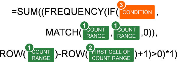
The image on the right-hand side shows the structure of the FREQUENCY formula with one condition. As you can see, the formula hasn’t changed much. Just one part is added, illustrated with number 3. You insert the condition using the IF formula. The corresponding closing blanket of the IF formula is after the MATCH formula. If the condition is not met, this part of the formula returns FALSE. This results in also FALSE at this point of the “DATA ARRAY” of the FREQUENCY formula.

Add the condition itself the following way: (CONDITION_RANGE=CONDITION)

The condition of our example table is to skip empty cells. The CONDITION_RANGE is A2:A11 and the condition is <>””. Putting the condition into the complete formula leads to the following formula.

=SUM((FREQUENCY(IF(B2:B11<>"",MATCH(A2:A11,A2:A11,0)),ROW(A2:A11)-ROW(A2)+1)>0)*1)

Adding the second criteria

After knowing how to handle one condition, it’s time to proceed with the second question of our example: How many people had a result higher than 40 in the first trial?

The same way the first condition is added, a second can be inserted. Just add one more IF formula before the existing IF formula. The corresponding closing bracket needs to be entered after the MATCH formula.

In the example of this chapter, the trial number is located in cells B2 to B11 and should be the first trial. The second criteria range is the result, located in cell range C2 to C11 and should be higher than 40. Regarding these two criteria leads to the following formula.

=SUM((FREQUENCY(IF(C2:C11>40,IF(B2:B11="1st trial",MATCH(A2:A11,A2:A11,0))),ROW(A2:A11)-ROW(A2)+1)>0)*1)

Once again, the hint: All formulas shown in this method are array formulas. After pressing Ctrl + Shift + Enter on the keyboard, curled brackets are added so that the formula―when seeing in the formula bar―look like this.

{=SUM((FREQUENCY(IF(C2:C11>40,IF(B2:B11="1st trial",MATCH(A2:A11,A2:A11,0))),ROW(A2:A11)-ROW(A2)+1)>0)*1)}

Method 6 (new). COUNTA and UNIQUE functions

Because the UNIQUE function is comparatively new in Excel, not all versions support this method. But because is by far the easiest, I have listed it first.

Just type the following function:

=COUNTA(UNIQUE(A:A))

in order to count the number of unique values in column A. Please note: A blank cell is also counted as one cell. If you don’t want to include blank cells in your counting, please extend the function like this:

=COUNTA(UNIQUE(A:A))-IFERROR(MIN(1,COUNTBLANK(A:A)),0)

Download

Please feel free to download all examples above in this Excel workbook. Click here and the download starts.

Image by RitaE from Pixabay