How to Return the Column Letter (Not Number) With Excel Function

There are a few cases in Excel when you need to return the column letter from an Excel cell. For example, when you use the INDIRECT function. Retrieving the number of a cell is quite simple using the =COLUMN() function. But the letter? Here is how to do that!

Summary

In a hurry? Copy and paste this function and replace “B5” with the cell you want to return the column letter from:

=SUBSTITUTE(ADDRESS(1,COLUMN(B5),4),"1","")

Introduction: Return the column number

Before we start, a small introduction of the simple =COLUMN() function in Excel. It returns the column number and is quite simple:

=COLUMN(B5)

This function returns the column number of cell B5 – so the result is 2 because column B is the second column.

You can also use this function without any argument:

=COLUMN()

This way, the function returns the column number of the current column.

Built-in Excel function to return the column letter from cell

We have seen above how to return the column number. Let’s take the next step now and return the column letter. I’m going to introduce you to the easiest method – of course, there are multiple options.

This version involves the ADDRESS function as well as the SUBSTITUE function. With the ADDRESS function we return the column letter as well as number and with the SUBSTITUTE function we remove the number from it.

The whole function is:

=SUBSTITUTE(ADDRESS(1,COLUMN(B5),4),"1","")

The key of this function is that the ADDRESS function converts the “coordinates” of a cell to letter and number. So, let’s only talk about the ADDRESS function now:

1. The first argument (1) is the row number. We set it to row number 1 and later on remove it with the SUBSTITUTE function.
2. As seen above, the COLUMN(B5) argument returns two and defines the column number in the ADDRESS function.
3. The number 4 as the third argument just defines the address style. Number 4 means a relative reference without any dollar signs.

That means, the ADDRESS function in this case returns “B1”. With the SUBSTITUTE function wrapped around we remove the one so that the final result is only “B”.

If you want to return the column letter of the current column, you can simply remove the B5. The function is:

=SUBSTITUTE(ADDRESS(1,COLUMN(),4),"1","")

Even easier: Use Professor Excel Tools to return the column letter

If you have Professor Excel Tools already, you can simply use the =PROFEXColumn() function to return the column letter.

In this case, it is:

=PROFEXColumn(B5)

For using the PROFEX functions you don’t have to purchase a license. In order to maximize the compatibility, all functions starting with =PROFEX are free to use.

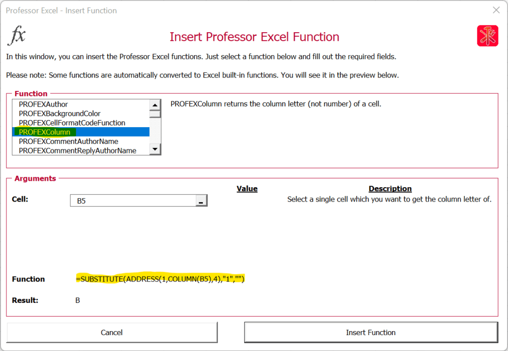
Even better: If you click on the fx button on the Professor Excel ribbon and insert the function here, it will automatically converted to built-in Excel function:

Please feel free to download Professor Excel Tools here for free. For more information, please click here.

Image by Lubos Houska from Pixabay