
Excel is a great software. It’s easy to use (at least the basic functions…) and very flexible. Unfortunately, coming with the flexibility, users tend to misuse the options and disobey certain basic rules. One thing I’ve seen multiple times is to transport important information in the formatting of a cell. It might be the background color, font color or strike-through. In this article, we’ll talk about something related: Return number format codes.
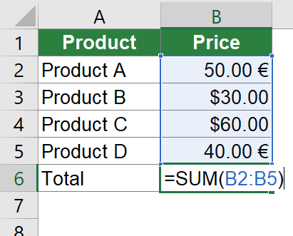
Let’s assume the following example. You receive a table containing prices with two columns. The first column contains the name of the item, for example “Product A”. The second column contains the respective prices. The problem is that instead of having one common currency, the currency information is only given in the number format code. Learn four methods in this article of how to return number format codes in Excel.
Please note: If you want to know how to use custom number format codes, please refer to this article. On this page we only explore how to return number format codes.
Method 1: Write the number format code manually
Our example above only has four rows so it’s quite fast to write the currency manually into a new column. But what if you Excel file has hundreds or thousands of rows?
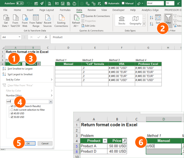
In such case, it might be helpful to use a filter. Filters show the format as displayed. So if the cell has “50 USD”, you can filter for USD although USD is only given in the number format code. Follow these steps.
- Add a filter to your data. In order to achieve this, select your table…
- …click on Data and then on Filter.
- Open the drop-down of the column containing the cell formats you want to read out.
- Type the number format code you want to filter in the search field, in this example “usd”.
- Confirm the filter with OK.
- Select a column on the right and type “USD”. Confirm with Ctrl + Enter.
Repeat steps 3 to 6 for the next number format code, for example “EUR”.
This is a straight-forward way to extract the most important information from the number format codes. Of course, this method comes with some disadvantages: The method might be fast on a single sheet and a limited number of number format codes to return. For larger workbooks, there are probably more efficient ways. Moreover, manual methods in Excel are later on or for other users usually not replicable. And last but not least, an update of your data requires to repeat the steps as shown above.
Method 2: Use the “CELL” formula to return the number format code
Excel has a built-in formula to return the number format code in Excel. The cell formula does that. You probably wonder, why it’s only the second of our four methods and why do we still need three other methods? The answer is simple: The CELL() formula returns crap often not sufficient results.
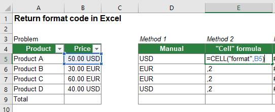
Let’s start of how to use the CELL formula. Just type =CELL(“format”,B5) if your cell with the number format code is B5. All well and good so far.
The problem: Not the number format code is returned but rather the “Text value corresponding to the number format of the cell.” And – as you can see from our example above – can be the same for different custom number format codes because it doesn’t include the custom text in the format code. Instead, you just get the superior number format category number.
It’s possible that this could solve your problem already, but often it doesn’t. It’s worth a try though. Please keep in mind the disadvantages that CELL is volatile and has problems with localisations (the formula does not adapt to your local language).
For more information, please refer to this support article from Microsoft.
Method 3: Insert a VBA Macro to return the cell format code
As so often with rather tricky problems in Excel, VBA can help. In this case, just 3 lines of code could be the solution.
Follow these steps.
- Insert a new VBA module (please refer to this article and scroll down to “How to insert a new VBA module manually” if you need more information).
- Copy and paste the following codes.
- Back in Excel, type =ProfessorExcelReturnCustomNumberFormatCode(B5) if you want to return the number format code from cell B5.
Function ProfessorExcelReturnCustomNumberFormatCode(cell As Range)
    ProfessorExcelReturnCustomNumberFormatCode = cell.NumberFormatLocal
End Function
Please note: This function returns locally-formatted strings and in the language used for the Office UI (or Windows version). If you want to return strings according to US number and date formats and English text, please replace cell.NumberFormatLocal by cell.NumberFormat (delete the local) in the end of the second line.
Method 4: Use Excel add-in
The most comfortable way to return the number format code is probably using an Excel add-in. I – of course – recommend my own add-in. You can download the free trial and even after expiring, the formula features still work.
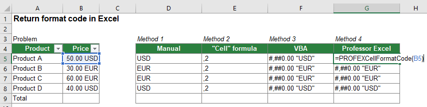
If you use the Professor Excel Tools add-in, just type =PROFEXCellFormatCode(B5). That’s it.

This function is included in our Excel Add-In ‘Professor Excel Tools’
(No sign-up, download starts directly)
More than 35,000 users can’t be wrong.
Download example workbook

Please feel free to download the example used in this article in this workbook.
Do you want to boost your productivity in Excel?
Get the Professor Excel ribbon!

Add more than 120 great features to Excel!