There are many cases in which you need a 2 dimensional lookup. That means, if you want to get a value from a specific row-column combination with neither rows or columns fixed. Unfortunately, the problem of a two way lookup comes up quite often. In this article we explore 4 methods of how to conduct 2D lookups in Excel.

+++NEW+++NEW+++NEW+++ 2D XLOOKUP +++NEW+++NEW+++NEW+++

In a hurry?

Most common for 2D lookups are INDEX/MATCH/MATCH (see method number 4 below) or a 2D XLOOKUP (click here for more information).

What is a 2D lookup?

At 2D lookups, you search for the row and column at the same time.

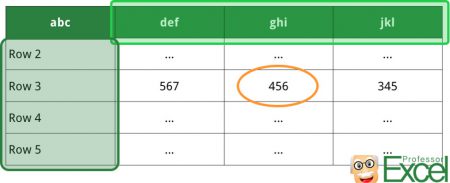
In many cases, you only look for a value in – let’s say – column A and return the corresponding value from column B. But there are also many examples, in which you don’t know the return column. For example, depending on the specifications, you want to return the value from either column B, C or D and so on. In such case, we are speaking of 2D lookups or a two way lookup. So we search in both rows and columns at the same time.

Preparations: The basic formulas for 2D lookups

The following methods are based on 4 basic formulas in Excel. Each formula we’ve described before, so please refer to these articles:

• VLOOKUP
• INDEX/MATCH
• INDIRECT
• HLOOKUP

The four methods

Example: Our table contains 3 data types for each country: The number of inhibitants, the VAT and the currency.

Before we jump in with the four methods, let’s take a look at our example first.

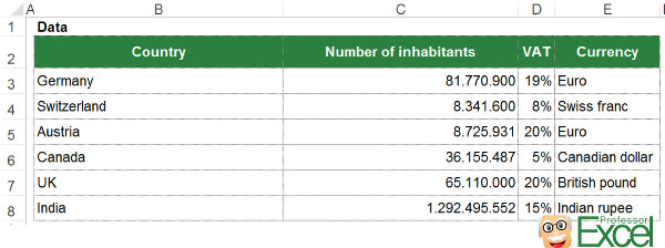
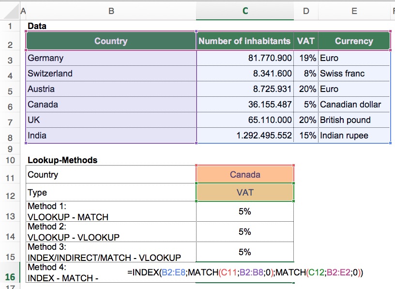
You got the simple table as shown in the image. In has data for different countries. For each country there are 3 types of data: The number of inhabitants, the VAT as well as the currency.

Solution: The overview of the four methods.

The task: Depending on the country and the data type you want to get the correct value from the table. For example, you select “Canada” and “VAT”, you want to get 5% in return.

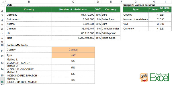
Below this table, we want to be able to define the country in cell C11 (here: “Canada”) and the data type in cell C12 (here: “VAT”). Depending on the combination, we want to retrieve the correct value from the data table above.

Method 1: The easiest way (VLOOKUP & MATCH)

Method 1: The VLOOKUP/MATCH combination.

Probably the easiest – or at least the shortest – way of returning values in 2 search dimensions is the VLOOKUP and MATCH combination. We start by setting up a normal VLOOKUP. But instead of setting a fixed value for the return column we use the MATCH formula finding the return column.

The formula in our example looks like this:

=VLOOKUP(C11,B2:E8,MATCH(C12,B2:E2,0))

The MATCH formula searches for the type, e.g. VAT, within the range B2 to E2. It returns the number of cell, in which it first comes up.

Closely related is a slightly different version: HLOOKUP with the MATCH formula. The HLOOKUP searches for “VAT” in the first row (row 2) and the match defines the number of the return row. =HLOOKUP(C12,B2:E8,MATCH(C11,B2:B8,0))

Method 2: You want to stay with VLOOKUP? (VLOOKUP & VLOOKUP)

Support table with column numbers for the VLOOKUP formula.

You are not familiar with the MATCH formula and just want to stay with VLOOKUP, you could go with this solution. We start the same way as in method one: We prepare the VLOOKUP formula for searching for the country name in column B. Instead of the return column number (“col_index_num”) we insert another VLOOKUP.

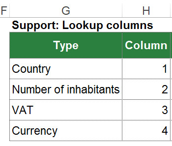
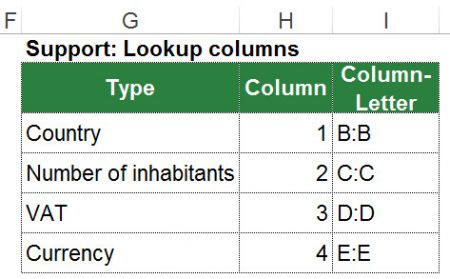
At this step, we need one more preparation. We set up a lookup table with the titles of your data. The second column (column H in the image) contains the number of column starting with 1 for the first title (in our case the country). The second VLOOKUP searches within this table and returns the number of columns.

The complete formula for the 2D Lookup looks like this:

=VLOOKUP(C11,B2:E8,VLOOKUP(C12,G:H,2,FALSE),FALSE)

---

Excel too slow? Speed it up. Get the book now!

Tired of waiting for Excel? Use the 30 best methods described in this book to speed up Excel calculations!

• Learn how Microsoft Excel performs calculations
• Use the simple and effective step-by-step guide to master each method
• Get to know the impact each method will have on performance

Learn more or get it on Amazon!

---

Method 3: The inconvenient way (INDEX & INDIRECT & VLOOKUP & MATCH)

Support table with column letters.

The third method is not really convenient as it is quite long. We’ve added it here is it shows an approach using the INDIRECT formula. You can transfer it – if you like – to the SUMIFS formula.

We need a bit more preparation for this method. We extend the support table from our method 2 above by the column letter (e.g. VAT = D:D). In order to keep it simple, we don’t simply write D but D:D as this is the complete return range.

In case of the VAT, the normal INDEX/MATCH approach without a dynamic search column would look like this: =INDEX(D:D,MATCH(C11,B:B;0))

With the MATCH formula we search for “Canada” in column B. It returns the number of the first occurrence of “Canada” within this range.

Now – in order to make also the return column a variable – you insert the INDIRECT formula and replace the “D:D”:

=INDEX(INDIRECT(VLOOKUP(C12,G2:I6,3,FALSE)),MATCH(C11,B:B,0))

That way, you search within the support table for “VAT”. Once found, it returns “D:D”. With the INDIRECT formula you really make it a part of the INDEX formula and can refer to the range “D:D”.

Method 4: The elegant way for 2D lookups: INDEX / MATCH / MATCH

Method 4: The INDEX/MATCH/MATCH combination.

This is probably the most elegant and most popular way for 2D lookups in Excel: Using the INDEX/MATCH/MATCH combination. Instead of just a simple INDEX/MATCH combination, you can add one more dimension with the second MATCH. The formula looks like this:

 =INDEX(B2:E8,MATCH(C11,B2:B8,0),MATCH(C12,B2:E2,0))

The INDEX formula has 3 parts here: The complete cell range (B2 to E8) and two MATCH formulas.

1. The return cell range stretches over the hole table. In our case that’s B2 to E8.
2. The first MATCH searches within the range B2 to B8 for the country.
3. The second MATCH looks for the type in the cell range B2 to E3 (the headline).

Both MATCH formulas return the number of the cell in with the search term the first time comes up.

Please feel free to download the example file here.

Method 5 (new): 2D XLOOKUP

Excel now has a new function – XLOOKUP. It’s offers a great alternative to the INDEX/MATCH/MATCH 2D lookup. Check it out here.

Bonus: How to change from percentage to normal number?

The cell is formatted as % when VAT is selected – otherwise “normal” number.

Use a conditional formatting rule for changing the %-sign when you display the VAT.

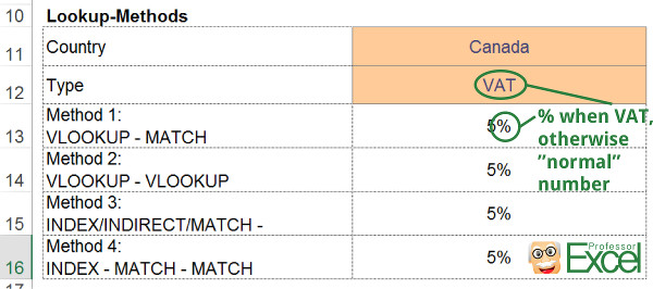
You’ve probably noticed, that in our example for the 2D lookups, the format of the return cell changes depending on the type of value. For instance, when you retrieve the value for VAT, the return cell is formatted with the %-sign. For other values, it shows normal number formats.

Follow these steps:

1. First step: Set the format of cell C13 to “Number”. In our case, we also use thousand separators. Text is still shown as text so we already got the value types “Number of inhabitants” and “Currency” covered.
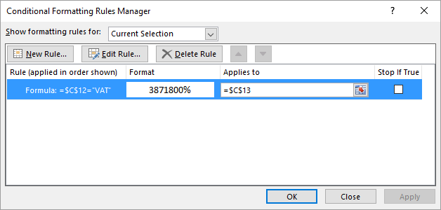
2. We only have to set up the exception for “VAT”. This can be done with conditional formatting. Click on “Conditional Formatting” in the center of the Home ribbon. Then click on “New Rule”.
3. In the lower dropdown list, choose “Use a formula to determine which cells to format”.
4. The condition is quite straightforward: =$C$12=”VAT”.
5. Define the format if your condition is true. In our case: Number format “Percentage”.
6. Click “OK”.

Please refer to this article for more information about conditional formatting with formulas.

Please note: Changing the number format with conditional formatting only works with Excel for Windows. As of now, this option is missing in the Mac version.